Excel 2010 - Outlining Data

Introduction

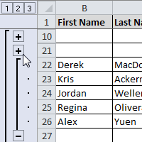
If the amount of data in your worksheet becomes overwhelming, creating an outline can help. Not only does this allow you to organize your data into groups and then show or hide them from view, but it also allows you to summarize data for quick analysis using the Subtotal command (for example, subtotaling the cost of office supplies depending on the type of product).

In this lesson, you will learn how to outline your worksheet in order to summarize and control how your data is displayed.

Outlining data

Outlines give you the ability to group data you may want to show or hide from view, as well as to create a quick summary using the Subtotal command. Because outlines rely on grouping data that is related, you must sort before you can outline. 

To outline data using Subtotal:

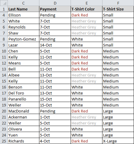
1. Sort according to the data you want to outline. Outlines rely on grouping data that is related. In this example, we will outline the worksheet by T-Shirt Size, which has been sorted from smallest to largest.
   
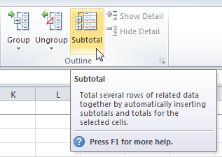
2. Select the Data tab, then locate the Outline group.
3. Click the Subtotal command to open the Subtotal dialog box.
   
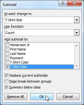
4. In the At each change in field, select the column you want to use to outline your worksheet. In this example, we'll choose T-Shirt Size.
5. In the Use function field, choose from the list of functions that are available for subtotaling. We'll use the COUNT function to tally the number of each size.
6. Select the column you want the subtotal to appear in. We'll choose the T-Shirt Size column.
7. Click OK.
   
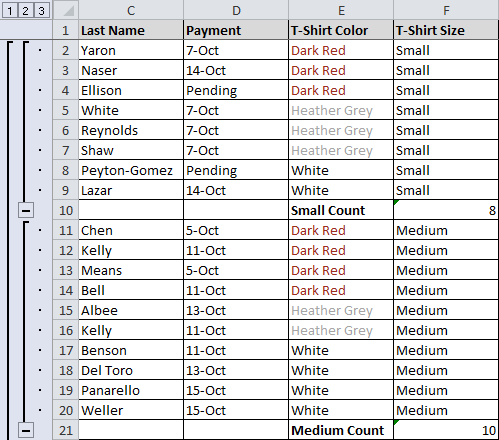
8. The contents of your worksheet will be outlined. Each T-shirt size will be placed in its own group, and the subtotal (count, in this case) will be listed below each group.
   

Showing and hiding data

To show or hide a group:

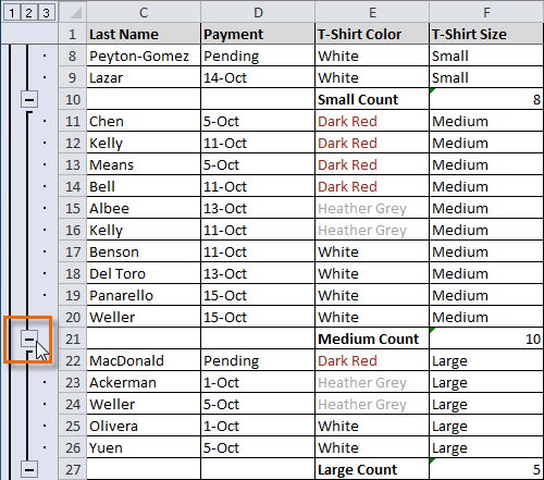
1. Click the minus sign—also known as the Hide Detail symbol—to collapse the group.
   
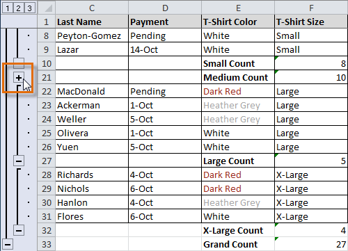
2. Click the plus sign—also known as the Show Detail symbol—to expand the group again.
   

You can also use the Show and Hide Detail buttons on the Data tab in the Outline group. Select a cell in the group you want to show or hide, then click the appropriate command.

To view groups by level:

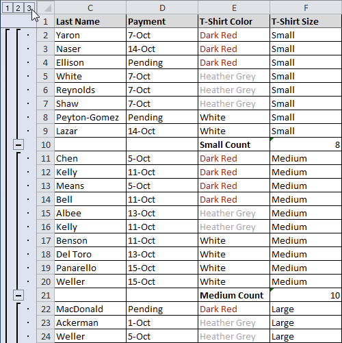
1. Click the highest level (level 3 in this example) to view and expand all of your groups. Viewing groups at the highest level will display the entirety of your worksheet.
   
2. Click the next level (level 2 in this example) to hide the detail of the previous level. In this example, level 2 contains each subtotal.
   
3. Click the lowest level (level 1 in this example) to display the lowest level of detail. In this example, level 1 contains only the grand total.
   

Removing groups and subtotaling

To ungroup data:

1. Select the rows or columns you want to ungroup. In this example, we'll ungroup size Small.
   
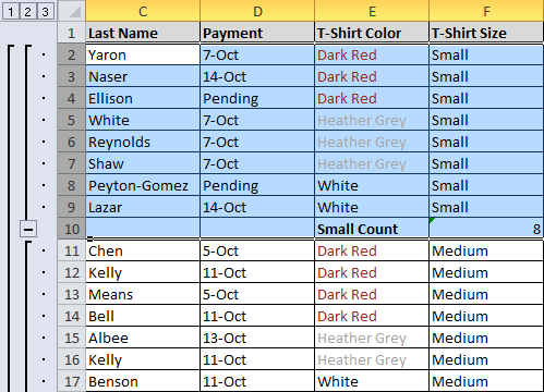
2. From the Data tab, click the Ungroup command. The range of cells will be ungrouped.
   

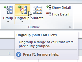
To ungroup all of the groups in your outline, open the drop-down menu under the Ungroup command, then choose Clear Outline.

Ungroup and Clear Outline will not remove subtotaling from your worksheet. Summary or subtotal data will stay in place and continue to function until you remove it.

To ungroup data and remove subtotaling:

1. From the Data tab, click the Subtotal command to open the Subtotal dialog box.
2. Click Remove All.
   
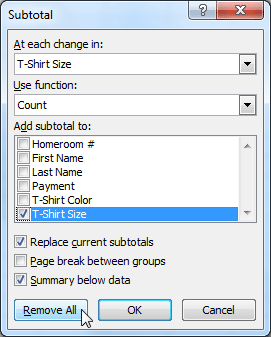
3. All data will be ungrouped, and subtotals will be removed.
   

Creating your own groups

The Group command allows you to group any range of cells—either columns or rows. It does not calculate a subtotal or rely on your data being sorted. This gives you the ability to show or hide any part of your worksheet and display only the information you need.

To create and control your own group:

In this example, we will prepare a list of T-shirt colors and sizes that need to be distributed to each homeroom. Some of the data in the worksheet is not relevant to the distribution of T-shirts; however, instead of deleting it, we'll group it, then temporarily hide it from view.

1. Select the range of cells you want to group. In this example, we will group the First Name, Last Name, and Payment columns.
   
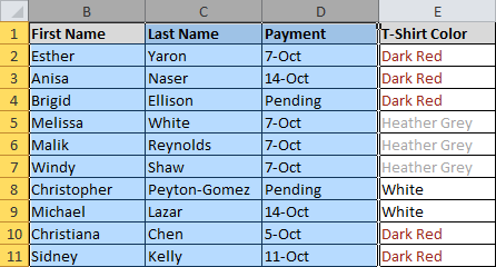
2. From the Data tab, click the Group command.
   
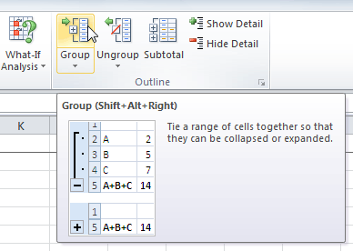
3. Excel will group the selected columns or rows.
   
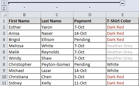
4. Click the minus sign—also known as the Hide Detail symbol—to hide the group.
5. The group will be hidden from view.

   

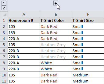
Click the plus sign—also known as the Show Detail symbol—to show the group again.

Challenge!

1. Open an existing Excel 2010 workbook. If you want, you can use this example.
2. Outline your worksheet using the Subtotal command. If you are using the example, outline by T-shirt size.
3. Display the first level of groups in your outline.
4. Display the highest level to view your entire worksheet again.
5. Create your own group of rows or columns, then hide the group from view.
6. Ungroup any range of data.
7. Remove subtotaling from your worksheet.