Excel 2010 - Using Conditional Formatting

Introduction

 Excel gives us several tools that will make this task easier. One of these tools is called conditional formatting. With conditional formatting, you can apply formatting to one or more cells based on the value of the cell. You can highlight interesting or unusual cell values, and visualize the data using formatting such as colors, icons, and data bars.

In this lesson, you'll learn how to apply, modify, and remove conditional formatting rules.

To create a conditional formatting rule:

1. Select the cells you want to add formatting to.
2. In the Home tab, click the Conditional Formatting command. A drop-down menu will appear.
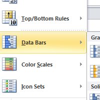
3. Select Highlight Cells Rules or Top/Bottom Rules. We'll choose Highlight Cells Rules for this example. A menu will appear with several rules.
4. Select the desired rule (Greater Than, for example).
   
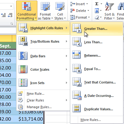
5. From the dialog box, enter a value in the space provided, if applicable. In this example, we want to format cells that are greater than $5000, so we'll enter 5000 as our value. If you want, you can enter a cell reference instead of a number.
6. Select a formatting style from the drop-down menu.
   
7. The formatting will be applied to the selected cells.
   

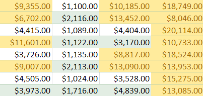
If you want, you can apply more than one rule to your cells.

Conditional formatting presets

Excel has several presets you can use to quickly apply conditional formatting to your cells. They are grouped into three categories:

• Data bars are horizontal bars added to each cell, much like a bar graph.
  
• Color scales change the color of each cell based on its value. Each color scale uses a two- or three-color gradient. For example, in the Green-Yellow-Red color scale, the highest values are green, the average values are yellow, and the lowest values are red.
  
• Icon sets add a specific icon to each cell based on its value.
  

To use preset conditional formatting:

1. Select the cells you want to add formatting to.
2. In the Home tab, click the Conditional Formatting command. A drop-down menu will appear.
3. Select Data Bars, Color Scales, or Icon Sets. Then select the desired preset.
   
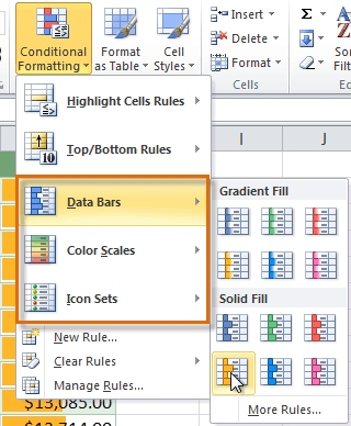
4. The conditional formatting will be applied to the selected cells.
   

To remove conditional formatting rules:

1. Select the cells that have conditional formatting.
2. In the Home tab, click the Conditional Formatting command. A drop-down menu will appear.
3. Select Clear Rules.
4. A menu will appear. You can choose to clear rules from the Selected Cells, Entire Sheet, This Table, or This PivotTable. In this example, we'll clear rules from the entire sheet.
   

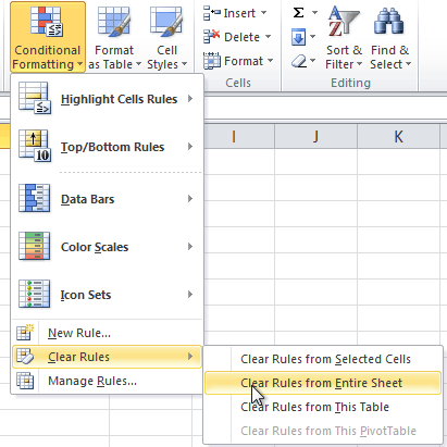
You can edit or delete individual rules by clicking the Conditional Formatting command and selecting Manage Rules. This is especially useful if you have applied multiple rules to the cells.

Challenge!

1. Open an existing Excel 2010 workbook. If you want, you can use this example.
2. Apply conditional formatting to a range of cells with numerical values. If you are using the example, apply formatting to all of the sales data.
3. Apply a second conditional formatting rule to the same set of cells.
4. Explore the Conditional Formatting Rules Manager dialog box.
5. Clear all conditional formatting rules from the worksheet.