Excel 2010 - Worksheet Basics

Introduction

Every Excel workbook contains at least one or more worksheets. If you are working with a large amount of related data, you can use worksheets to help organize your data and make it easier to work with.

In this lesson, you will learn how to name and add color to worksheet tabs, as well as how to add, delete, copy, and move worksheets. Additionally, you will learn how to group and ungroup worksheets and freeze columns and rows in worksheets so they remain visible even when you're scrolling.

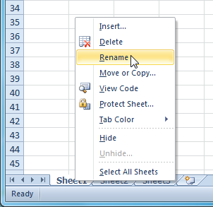
To rename worksheets:

1. Right-click the worksheet tab you want to rename. The worksheet menu appears.
2. Select Rename.
   
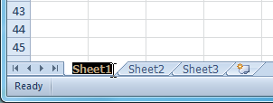
3. The text is now highlighted by a black box. Type the name of your worksheet.
   
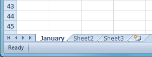
4. Click anywhere outside the tab. The worksheet is renamed.
   

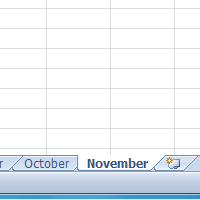
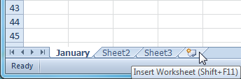
To insert new worksheets:

Click the Insert Worksheet icon. A new worksheet will appear.

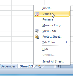
To delete worksheets:

1. Select the worksheets you want to delete.
2. Right-click one of the selected worksheets. The worksheet menu appears.
3. Select Delete. The selected worksheets will be deleted from your workbook.
   

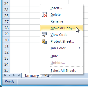
To copy a worksheet:

1. Right-click the worksheet you want to copy. The worksheet menu appears.
2. Select Move or Copy.
   
3. The Move or Copy dialog box appears. Check the Create a copy box.
   
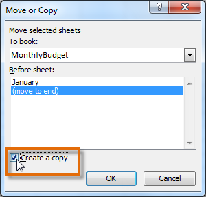
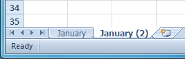
4. Click OK. Your worksheet is copied. It will have the same title as your original worksheet, but the title will include a version number, such as January (2).
   

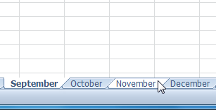
To move a worksheet:

1. Click the worksheet you want to move. The mouse will change to show a small worksheet icon .
2. Drag the worksheet icon until a small black arrow appears where you want the worksheet to be moved.
   
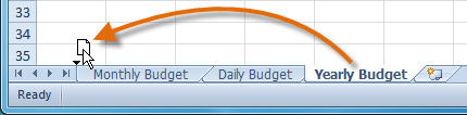
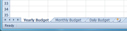
3. Release your mouse, and the worksheet will be moved.
   

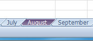
To color code worksheet tabs:

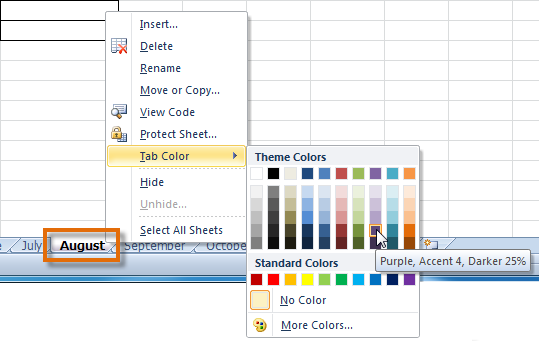
1. Right-click the worksheet tab you want to color. The worksheet menu appears.
2. Select Tab Color. The color menu appears.
3. Select the color you want to change your tab.
   
4. The tab color will change in the workbook. If your tab still appears white, it is because the worksheet is still selected. Select any other worksheet tab to see the color change.
   

To group worksheets:

1. Select the first worksheet you want in the group.
   
2. Press and hold the Ctrl key on your keyboard.
3. Select the next worksheet you want in the group. Continue to select worksheets until all of the worksheets you want to group are selected.
   
4. Release the Ctrl key. The worksheets are now grouped. The worksheet tabs appear white for grouped worksheets.

To ungroup all worksheets:

1. Right-click one of the worksheets. The worksheet menu appears.
2. Select Ungroup. The worksheets will be ungrouped.

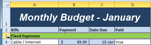
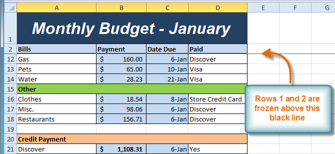
To freeze rows:

1. Select the row below the rows you want frozen. For example, if you want rows 1 and 2 to always appear at the top of the worksheet even as you scroll, then select row 3.
   
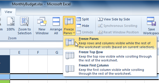
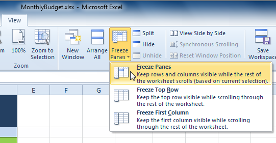
2. Click the View tab.
3. Click the Freeze Panes command. A drop-down menu appears.
4. Select Freeze Panes.
   
5. A black line appears below the rows that are frozen in place. Scroll down in the worksheet to see the rows below the frozen rows.
   

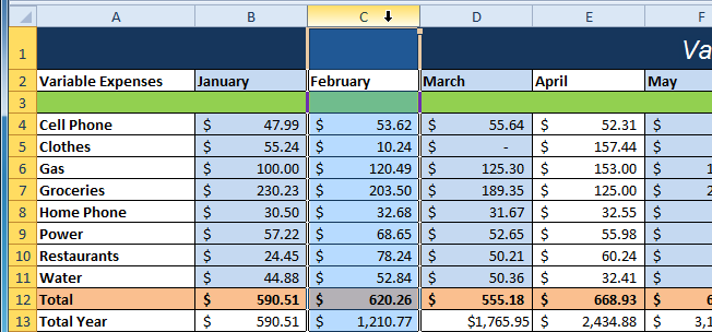
To freeze columns:

1. Select the column to the right of the columns you want frozen. For example, if you want columns A and B to always appear to the left of the worksheet even as you scroll, select column C.
   
2. Click the View tab.
3. Click the Freeze Panes command. A drop-down menu appears.
4. Select Freeze Panes.
   
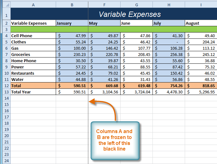
5. A black line appears to the right of the frozen area. Scroll across the worksheet to see the columns to the right of the frozen columns.
   

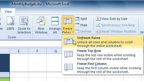
To unfreeze panes:

1. Click the View tab.
2. Click the Freeze Panes command. A drop-down menu appears.
3. Select Unfreeze Panes. The panes will be unfrozen, and the black line will disappear.
   

Challenge!

1. Open an existing Excel 2010 workbook. If you want, you can use this example.
2. Insert a new worksheet.
3. Change the name of a worksheet.
4. Delete a worksheet.
5. Move a worksheet.
6. Copy a worksheet.
7. Try grouping and ungrouping worksheets.
8. Try freezing and unfreezing columns and rows.